More Thoughts on the Welfare Consequences of Stimulus Spending

Noah Smith has a short post questioning the reasoning of an earlier post of mine about stimulus spending. He includes a short numerical example which I reproduce below.  Here’s Noah:

Suppose [the] fiscal “multiplier” is substantial. Specifically, suppose … $100 of tax rebates will increase GDP by $110. In this case, stimulus spending is a “free lunch.”

Now suppose that instead of doing tax rebates, the government can build a bridge. The social benefit of the bridge is $90, and the bridge would cost $100. In the absence of stimulus effects, therefore, the bridge would not pass a cost-benefit analysis. For simplicity’s sake, suppose that spending money on the bridge would create exactly the same stimulus effect as doing a tax rebate – spend $100 on the bridge, and GDP goes up by $110 from the stimulus effect.

In this case, the net social benefit of spending $100 building the bridge is $90 + $110 – $100 = $100.
And the net social benefit of spending $100 on a tax rebate is $110 – $100 = $10.

Bridge wins!

Noah has a couple of subtle mistakes in his calculation. First, the increase in GDP from the stimulus isn’t completely a social benefit. Typically, every good produced is produced at some cost. If I go out to eat for lunch and buy $10 of Szechuan chicken, GDP goes up by $10. However, the net social benefit doesn’t go up by this amount. The gains to me (G) must be at least worth $10 otherwise I wouldn’t have willingly spent the money. The cost to the restaurant (C) can’t be more than $10 otherwise they wouldn’t have willingly provided that dish.  The social benefit (SB) is the difference between the gains and the cost.

SB = G – C

If markets are fairly competitive then at the margin both G and C will be “close” to $10 and so the social benefit will in all likelihood be less than $10. What this means for Noah’s calculation is that the $110 stimulus might not really be worth $110.  That’s ok however since this error is symmetric. It is worth pointing out however, that stimulus which is guided by the private sector typically passed cost/benefit tests of the kind I emphasize. In my example, G > 10 and C < 10 so SB = G – C must be positive. 

The second error is more important. In his calculation, Noah is counting the out-of-pocket revenue outlay for the tax cut as a cost. This isn’t correct. The tax cut is a transfer. There are no direct social costs associated with the tax cut.

Let me try to rephrase Noah’s example to make it clear. He is considering two options:

OPTION 1: tax cut (or transfer) of $100

OPTION 2: government spending of $100

(i) In both cases the Treasury is deprived of $100. 

(ii) In both cases the private sector gains $100 in after-tax income.

(iii) In both cases the private sector uses the additional income to spend or save (this is the source of the multiplier). 

(iv) In OPTION 1 a bridge is built. The social costs (C) of the bridge include the value of time, energy, materials, effort, etc. The social benefit (B) of the bridge is the value of having the bridge.

In comparing these two options, we can ignore (i) – (iii) since they are the same in both policies. The only difference is (iv). Whether government spending is preferable depends only on whether B is bigger than C.  Note that the magnitude of the multiplier doesn’t enter the comparison. It is symmetric in both cases. My argument is not “diametrically opposed to Econ 102 textbook Keynesianism” —  GDP will go up by more under OPTION 2.  The subtlety is that in Econ 102 we typically act as if maximizing GDP is the correct objective of public policy. This isn’t true though. GDP maximization can rationalize building pyramids, the Maginot Line, the bridge to nowhere, ethanol subsidies, … A social welfare criteria would skip these projects.

In the comments section to Noah’s post a number of readers make some points which are worth mentioning. One comment points out that many people don’t pay taxes and so wouldn’t benefit from a tax cut. Certainly, unemployed people won’t benefit from a tax cut. However, we could construct transfers that would reach these people. Rachel Maddow’s suggestion of sending people envelopes with money in them would work just fine. Also, many people and firms do pay taxes. Payroll tax cuts like those passed by the Obama administration are a particularly effective way of introducing stimulus.  These simultaneously put money in people’s pockets not to mention the beneficial incentive effects of the policy. 

Another commenter points out that calculating the social costs and benefits of a given project are quite difficult.  This is absolutely true but it is a calculation that should be carefully considered none the less.  In Noah’s example, the cost of bridge is probably closely approximated by $100.  The benefit of the bridge is more difficult to assess.  Such difficulties probably come up often.  What is the benefit of protecting or cleaning up a wetland?  What is the benefit of political stabilization in the Middle East? Tricky questions but questions that should be considered nonetheless. 

Are Agent-Based Models the Future of Macroeconomics?

A couple months back, Mark Buchannan wrote an article in which he argued that ABMs might be a productive way of trying to understand the economy.  In fact, he went a bit further – he said that ABMs would likely be the future of economics and he warned young economists not to get caught watching the paint dry and to get on board with this new approach to the study.  In contrast, he pointed to the failings of the DSGE models that mainstream economists use to understand most economic issues.

An AMB is a model environment computer model that is comprised of many individual participants. These actors interact with one another and these interactions produces outcomes – in our case, economic outcomes.  These economic outcomes can then be added up to compute GDP and aggregate, investment – any of the economic statistics that we macroeconomists are accustomed to looking at – you could calculate in an ABM.

Now, if you are an economist, a macroeconomist in particular, you are probably thinking that so far this sounds very familiar – it sounds like a DSGE model.  A DSGE model is populated by many agents and they interact and the results of those interactions produce economic outcomes and we add up those outcomes and we get GDP and so forth so it sounds like ABMs are DSGE models so how are they at all different?

Well, there are actually a few important differences.  More accurately, it seems to be a combination of three key differences that distinguishes the ABMs.

Probably the most important distinguishing feature is that, in an ABM, the interactions are governed by rules of behavior that the modeler simply encodes directly into the system individuals who populate the environment.[1] For example, we could have an ABM with a purely Keynesian consumption rule. We could assume that every time a consumer earns a dollar of income, they spend 20 cents and save the remaining 80 cents. We would make similar behavioral assumptions to govern every possible interaction.  We would make these assumptions for consumers, workers, firms, investors, etc. In an ABM, behavior is the point at which a modeler starts making assumptions.

People who write down DSGE models don’t do that. Instead, they make assumptions on what people want. They also place assumptions on the constraints people face. Based on the combination of goals and constraints, the behavior is derived.  The reason that economists set up their theories this way – by making assumptions about goals and then drawing conclusions about behavior – is that they are following in the central tradition of all of economics, namely that allocations and decisions and choices are guided by self-interest. This goes all the way back to Adam Smith and it’s the organizing philosophy of all economics. Decisions and actions in such an environment are all made with an eye towards achieving some goal or some objective. For consumers this is typically utility maximization – a purely subjective assessment of well-being.  For firms, the objective is typically profit maximization. This is exactly where rationality enters into economics. Rationality means that the “agents” that inhabit an economic system make choices based on their own preferences.

A second key difference is that the interactions are often restricted to individual (or at least limited) interactions. It could be a limited number of connections between a given consumer and potential sellers. It could be a single connection between a worker and a firm and so on.

Lastly, the individuals are “heavy.”  That is, the models keep track of each and every individual in the system and the behavior of each and every one matters (to some extent) to determine the outcome. This is again unlike many standard economic systems.  In most macroeconomic systems the behavior of a single individual can be altered without having a perceptible impact on the aggregate outcome. This isn’t typically the case in ABMs. In an ABM, one individual can influence the outcome at least to a degree.

Now, all of these features have been analyzed in economics. Macroeconomists have models that explore the consequences of matching (or search) in which the individuals make deals on a bilateral basis. In game theory, we often have environments in which each player has a substantial influence on the outcome. And there are well-known models that consider ad hoc rule-of-thumb behavior. However, these modifications are rarely considered in combination.

Of the three features, the absence of rationality is the most significant.  Ironically, eliminating rational behavior also eliminates an important source of feedback – namely the feedback from the environment to behavior.  This type of two-way feedback is prevalent in economics and it’s why equilibria of economic models are often the solutions to fixed-point mappings. Agents make choices based on the features of the economy.  The features of the economy in turn depend on the choices of the agents. This gives us a circularity which needs to be resolved in standard models. This circularity is cut in the ABMs however since the choice functions do not depend on the environment. This is somewhat ironic since many of the critics of economics stress such feedback loops as important mechanisms.

The absence of rational behavior also means that the ABMs are much easier to solve than traditional models. Once you have settled on your preferred choice functions, you just assemble many such individuals together in a computer environment and simply simulate.

In fact, the predecessors of ABMs have been around for quite a while. The earlier versions were called “cellular automata.”  The most famous of these was John Conway’s famous “Game of Life.” This “game” took place on a grid (often a torus).  Each square on the grid was either on or off (alive or dead). If a cell was alive at time t, it remained alive if 2 or 3 of its eight neighboring squares were also alive.  If 1 or 0 of its neighbors was alive then the cell “died” due to isolation.  If 4 or more were alive, the cell died due to congestion. Cells could also come to life. An inactive (dead) cell would come to life if it had exactly 3 live neighbors. The environment was very intricate. Starting from a random patter of active/inactive cells, a huge array of outcomes could be supported. There could be bursts of activity followed by a dramatic collapse.

In fact, you can get simple versions of cellular automata as apps on your iPhone. Two good ones are SPEED sim, and CA2D.  CA2D has many cellular automata rules built in but it doesn’t have the Game of Life.  Below are three pictures of Conway’s game of life taken from SPEED sim.  The first panel shows an initial purely random starting point. The second panel shows the system after 25 iterations. You can see that patterns have emerged “naturally” from the initial random state. The last frame shows the steady state.

Initial Random State

After 25 Iterations

Steady State (Periodic)

Clearly even in this simple ABM we can get very complicated patterns and behavior.

Whether ABMs have any future in economics is not clear. I suspect that the rule-based approach at the heart of the ABMs will ultimately limit their usefulness – particularly if outcomes depend importantly on subtle differences in specifications of the rules or if individuals have to adhere to simple rules even when the system starts acting wild.

Another problem facing the ABMs is that they appear to be suggested as a solution to a problem that might not exist.  In their 2009 Nature article, J. Doyne Farmer and Duncan Foley write that DSGE models “assume a perfect world, and by their very nature rule out crises of the type” we experienced in 2007-2008.  DSGE models do not “assume a perfect world.” Economists are enthusiastically adding frictions and modifications to DSGE models which incorporate many real-world types of market failures.  I will concede that I would be reluctant to offer a particular version of a DSGE model that I felt accurately captured what was going on during the crisis but I don’t think this is because of a limitation of the DSGE approach.  It’s a limitation of economists fundamental understanding of financial crises.  And that’s not something that ABMs are going to fix ….

[1] An attentive reader pointed out that my original description incorrectly described the rules as applying at the system level. This is incorrect. The rules of behavior are attached to the individuals and each can have a different rule. 

Paul Krugman’s View of Aggregate Demand and Aggregate Supply

Paul Krugman responds to my earlier post.  He has a lot to say that’s worth commenting on.  I think we actually agree on quite a bit though there are points where we disagree.  Let’s take a look. (Paul’s comments in italics).

As I see it, we [i.e., Keynesian macroeconomists] have a general proposition — most recessions are the result of inadequate demand.

I basically agree with this though I admit that I don’t have a particularly clear definition of what we really mean by “aggregate demand.”  I think often this is meant to capture changes in consumer sentiment, fluctuations in government demand for goods and services or other incentives to purchase market goods – incentives which would include tax subsidies, monetary stimulus, … etc.

[…] we have a pretty good model of aggregate demand, and of how monetary and fiscal policy affect that demand. That model is IS-LM, with endogenous money as appropriate. 

Again I basically agree, with the caveat that the IS-LM model is at most just a sketch.  The consumption block of the IS-LM model is much better treated by a modern consumption demand component augmented suitably with credit constraints, some hand-to-mouth behavior and perhaps some myopia.  The investment block needs some serious work. My own sense is that it is also much better handled with a modern formulation rather than a simple relationship between investment and the real interest rate.  I would also stress that while the IS-LM sketch is pretty good as it stands, it desperately needs to incorporate a serious treatment of the financial sector. In a sense there is a third market / third curve missing from the model – one which gives the interest rate / loan terms faced by consumers as a function of collateral, net worth, etc.  We would then get a lot closer to a sketch which could capture important elements of the financial crisis.  (See below for a more precise description.)

We do not have an equally good model of aggregate supply.

I completely agree.

What we have, instead, is an observation: prices and wages clearly are sticky in the short run, and maybe for longer than that. There’s overwhelming evidence for that proposition, but in trying to justify it we engage in various kinds of hand-waving about menu costs and bounded rationality.

On the evidence I am again in complete agreement.  I actually think Paul is being too dismissive of the justifications for why we see price and wage rigidity.  Macroeconomists have invested a huge amount of time and energy into studying price setting behavior and these studies give a pretty clear picture of what is going on at the “micro level.”  It’s not just hand-waiving.  Paul continues…

we can […] be fairly sure that expansionary policies in a depressed economy won’t be inflationary, and we can use the pretty good demand side model to tell us that monetary expansion won’t work but fiscal policy will when we’re at the zero lower bound.

I sort-of agree with this.  Certainly if the interest rate is zero then conventional monetary expansions won’t do anything.  Whether government stimulus is a good move is unclear.  I am sure that government spending increases employment and output to an extent but it is very important how the money is spent. In an earlier post I argued that even in a severely depressed economy, there is rarely a good justification for spending on projects that aren’t socially valuable.  In all likelihood the best fiscal policies will involve some sort of transfer (like payroll tax cuts) or other tax cut rather than government spending.

What the data actually look like is an oldfashioned non-expectations Phillips curve. 

OK, here is where we disagree.  Certainly this is not true for the data overall.  It seems like Paul is thinking that the system governing the relationship between inflation and output changes between something with essentially a vertical slope (a “Classical Phillips curve”) and a nearly flat slope (a “Keynesian Phillips Curve”).  I doubt that this will fit the data particularly well and it would still seem to open the door to a large role for “supply shocks” – shocks that neither Paul nor I think play a big role in business cycles.

Paul ends his post with some bait.  He writes “it remains true that Keynesians have been hugely right on the effects of monetary and fiscal policy, while equilibrium macro types have been wrong about everything.”  OK, I’m again going to try not to take the bait.  Let me just point out that this is a difficult statement to take very seriously.  For the most part, the Keynesians are a subset of the equilibrium types.  Moreover, there are many “equilibrium types” who are not Keynesian but who are instead finance guys who played a crucial role in analyzing the economy during the crisis.  I presume he is taking an obligatory shot at Minnesota / Sargent / Lucas / Mathematical modelling etc. but …. I’m not taking the bait.

 

APPENDIX: The traditional IS-LM system is something like this:

Y = C(Y,r) + I(r) + G +NX(e)

r = max{-π, aY + b(π) }

the first equation is the IS curve governing the goods market. Consumption demand is increasing in Y and decreasing in r.  Investment demand is decreasing in r and Net Export demand is a function of the (real) exchange rate.  The second equation is the LM curve which I have written as a Taylor rule with the restriction that the nominal interest rate (i  = r – π) is subject to the ZLB.

A simple improvement over this system would be to introduce a different borrowing rate for firms and households – call this rate R.  R is equal to the base rate r plus an “external finance premium.” The EFP could be a decreasing function of asset values A and income Y. We now have the modified system

Y = C(Y,R) + I(R) + G +NX(e)

r = max{-π, aY + b(π) }

R = r + EFP(Y, A)

I’ll call the third equation the FE curve since it provides a condition for financial market equilibrium.  This model will have a spread R-r which will reflect financial stress.  Of course the IS-LM-FE system is again just a sketch.  We still have no explicit role for liquidity, solvency concerns, bank runs, etc. and the FE block would need to be fleshed out.  In fact this model is essentially a static sketch of the financial accelerator model by Bernanke, Gertler and Gilchrist 1999.

Traditional Macroeconomic Models and the Great Recession

A common narrative: analysts who used traditional Keynesian tools to understand the crisis made better predictions and were in a better position to diagnose the problem. This narrative may be comforting to some but unfortunately it’s not correct.

In some sense, the truth of our predicament is even scarier. Macroeconomists were caught completely off-guard by the financial crisis. None of the models we were accustomed to use provided insights or policy recommendations that could be used for fighting the crisis. This is particularly true for New and Old Keynesian models. The New Keynesian model (particularly its DSGE manifestations) was the dominant macroeconomic paradigm in the pre-crisis period and judging by many of the presentations at the National Bureau of Economic Research (NBER) summer meetings, the New Keynesian or Old Keynesian (referred to as “paleo Keynesian” by some of the meeting participants) continue to serve as the primary lens through which we try to make sense of the macroecononmy.

It its standard form, neither the New Keynesian model nor its paleo-Keynesian antecedent feature a meaningful role for financial market failures. As a result, the policy response to the crisis was largely improvised. This is not to say that the improvised policy actions were bad. Improvisation guided by Ben Bernanke was about as good as we could hope for. Nevertheless, for the most part, the models we were accustomed to use to deal with business cycle fluctuations were simply incapable of making sense of what was going on. In one of Stefanie Kelton’s recent podcasts, economist Randy Wray makes exactly this point. While I typically do not grant much credence to heterodox economists, in this instance Professor Wray’s diagnosis is completely correct. Fortunately, as Noah Smith pointed out in an earlier column,macroeconomists have been working, and continue to work, on developing models that can be used to analyze financial market failures.

In addition to the fact that the prevailing business cycle theories did not incorporate financial sectors, the components that were featured prominently were not performing well. The cornerstone of pre-crisis macroeconomic theory was price rigidity. In New Keynesian models, price rigidity results in a Phillips curve relationship – more specifically, a New Keynesian Phillips curve. According to the Phillips curve, if inflation was unusually high then output would be above trend. If it was low then output would be below trend.

The financial crisis of 2007-2008 and the Great Recession that followed proved to be a particularly bad episode for the New Keynesian model. Contrary to Paul Krugman’s assertion that traditional Keynesian models performed well, the key mechanism in the New Keynesian framework – the Phillips curve – was a virtual failure. In a recent post commenting on John Cochrane, Noah Smith plots quarterly price growth during the recession and notes that inflation did fall a bit during the recession. In his words “inflation not only plunged during the recession, but remained low after the recession.” The chart below shows core inflation (inflation for all goods excluding food and energy) since 2004. Clearly inflation fell once the recession took hold. Prior to 2008 annual inflation had been roughly 2 percent. Inflation fell during the recession [1] to roughly 1 percent.

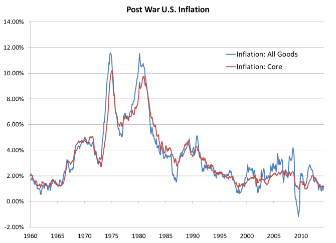
To put this change in perspective, the next chart plots annual inflation for the entire post-war period. The blue line is the inflation rate for all goods in the CPI. The red line is core inflation.

There have been many large swings in inflation during U.S. history. Compared to historical variations in inflation through the post-war, the changes in price growth during the Great Recession were quite mild. Notice that because the large drop in the overall inflation rate is not in the core measure, this movement reflects changes in food and energy (primarily oil prices). If the 1 percent reduction in core inflation is sufficient for the Keynesian model to generate the huge recession we just went through then where was the huge recession in the late 1990s? Where was the enormous recession in 1986?

In his 2011 AEA presidential address Bob Hall proposed modifying the Keynesian model by treating inflation as “nearly exogenous.” One might interpret this modification as a “hyper-Keynesian” element – the exogeneity of inflation arises because the Phillips curve is essentially flat so even minor variations in inflation cause sharp changes in output. Alternatively, one could interpret the modification as a capitulation of sorts. The inflation block of the model is incorrect and so Hall removed it, letting inflation march to its own beat, unaffected by developments within the system.

Traditional Liquidity Trap models predict that inflation should not only be low but it should be falling. Instead, even though interest rates were pushed to zero and even though economic activity contracted dramatically, the inflation rate barely budged. In his paper, Hall writes [of the New Keynesian Phillips curve] “luckily the theory is wrong.” Were the Phillips curve true, inflation would have fallen making the real interest rate even more negative, further depressing output and employment.

While commentators like Paul Krugman are correct to point to a few success stories of some models (like some aspects of the Liquidity Trap), they should also own up to the mounting evidence that the older models (even the paleo-Keynesian models that some prefer) clearly failed on some important dimensions. They couldn’t tell us much of anything about what caused the financial crisis itself and couldn’t really tell us how to deal with it and they made clear predictions about inflation that were supposedly at the center of the New Keynesian mechanism – predictions that never materialized.

 

 

[1] I am plotting the percent change in the price indices from year t-1 to year t.

Back to Blogging

Sorry for the long blogging hiatus.  I’m not immune to the tug of summer but  I will start posting again soon.

This week I am at the NBER summer institute in Boston MA.  There are many excellent research papers that I have seen so far this week and we still have two days to go.  The presentation by John Cochrane was particularly lively (not surprising given the controversial message of the paper).  

Fixing Terrible Economics Presentations II: Guide for the Audience

In an earlier post, I outlined several all-too-common flaws in economics seminar presentations. Those comments were directed toward the presenter. However, having a valuable seminar is not just the responsibility of the speaker — the audience shares in the experience and yes there are some guidelines for being a good seminar participant. I’m going to use this post to address some of the more troublesome infractions of seminar etiquette for participants.  

1. Read the paper in advance! — Just kidding. It’s quite common for seminar participants to go into a seminar “blind” so to speak. Not reading the paper isn’t a sin. If you can read it ahead of time that can be good but it shouldn’t be necessary if the presenter has done his or her job. You have the right to expect to go into a seminar and learn the main points of the paper without having to study the material ahead of time. There may be people who have read the paper before hand (people in the field who have personal reasons to know the paper thoroughly) but don’t feel bad if you aren’t one of them.  

2. Arrive on time! OK, this is a simple rule you can follow to improve the seminar for everyone. If you arrive late it disrupts the talk; you miss the introduction (which is often the key part of the talk) and you make it seem like you don’t really care. If something came up and you’re running late then fine, politely find a seat and try to catch up the best you can. If you are habitually late then you need to get your act together and show up on time.  

3. Try not to ask “exploratory” questions. An exploratory question is a question which doesn’t deal directly with the talk but instead asks the presenter to consider or comment on material which may not be in the paper. Suppose a presenter has just gone through the first slide of the model and someone asks “Have you considered what would happen if you added […] ?” This is probably not a good question at this point in a talk. There are basically two possibilities: (1) the speaker has considered this possibility and will get to it later in the talk or (2) the speaker hasn’t considered the possibility. If it’s (1) then the question only serves to delay the presentation and interrupt the flow. If it’s (2) then the question is either going to embarrass the speaker or it will get the speaker talking about something that isn’t in the paper. None of these outcomes is desirable.  Questions that are open-ended should be left for the end of the talk (assuming the speaker doesn’t address the question along the way). Keep a piece of paper to write down such questions and ask at the end if there is time.  

4. The questions you should ask are “clarifying questions.” These are questions which are intended to (duh) clarify. You misunderstood what the speaker just said. You didn’t understand how equation (iii) followed from (ii). You don’t understand the units of the graph. ASK. These questions are excellent because they help the audience understand the presentation (others almost surely had the same confusion). They serve to pace the talk. (Note, the speaker should have the correct answer to any clarifying question. If he or she doesn’t then they should be embarrassed.) 

5. Don’t ask so many questions (or “harp on” about an issue) that it makes it difficult for the presenter to get through the material. Let the presenter finish. If you ask a question but aren’t satisfied with the answer you can ask again after the talk. If you keep pressing the issue, you aren’t making progress you are just damaging the talk for everyone else. 

6. Finally, in the immortal words of the great Tom Brady, don’t be a turd! As a field, economics is nasty enough as it is. We really don’t need the audience acting like brats during seminars to add to the problem. I once spoke with an economist from a top program who actually boasted that, in his department, the audience was so aggressive that often the presenter didn’t make it out of the introduction. I pointed out that this was perhaps the dumbest thing I had ever heard and that it would be more efficient to simply not invite the speaker in the first place or perhaps you could lock the speaker in a visitors office — that way they wouldn’t even get to the introduction. If you are being hyper aggressive or nasty — particularly to a junior economist or to a graduate student — you really need to stop. It’s not productive. It doesn’t impress anyone. It compromises the value in the seminar. Worst of all — it gives other members of the audience the impression that this is acceptable behavior. It’s not. Don’t be a turd. 

Improving Econ 101

In a recent BloombergView article Noah Smith argues that the reason introductory economics classes are so bad is that they have few empirical demonstrations of their basic insights.  He draws a contrast between Econ 101 and introductory Physics classes.  While the physics classes actively demonstrated that their theories had merit, in Econ 101 and 102, 

… there were no demonstrations. There was basically nothing but theory — all the pretty little theories of comparative advantage and monopoly pricing and loanable funds, and not a whiff of evidence to back them up.

This observation leads Noah to conclude that introductory economics classes need a greater emphasis on empirics — much the way that the profession has shifted emphasis towards empirics recently.  

There might be some truth to Noah’s argument and his recommendation but I have some doubts all the same.  

Introductory economics – particularly introductory microeconomics – introduces students to, as Greg Mankiw summarizes it, “comparative advantage, supply and demand, market efficiency and market failure.”  That sounds about right but I would say that supply and demand reasoning is the most important tool the students are exposed to. Supply and demand models have a huge number of applications: labor markets, rental markets, the market for illicit drugs, the market for video rentals, the market for foreign currency, the market for short term lending, etc.  Moreover, there are many compelling empirical examples of supply and demand analysis in action. Obviously there is a huge literature on the effects of minimum wages which requires nothing more than supply and demand. There is a literature on rent control. There is the famous empirical study of labor markets (and capital markets) during the Black Death. There are empirical results on tax subsidies, tariffs, farm subsidies, … There are empirical studies of the market for banking reserves. Empirical studies of the effects of entry on prices (think jetBlue) and so on.  Instructors should definitely expose the students to these results — none of which are really new.  

I’m a bit surprised that Noah didn’t mention the increasing prevalence of in-class experiments. (I’m surprised because Noah’s Ph.D thesis focused on experimental analysis of asset pricing games). There are tons of fun in-class demonstrations that can be run.  In-class auctions, bank-run experiments, prisoner’s dilemma experiments, price ceiling experiments, and so forth. Students often really appreciate these demonstrations and they have a way of bringing to the material to life in the way that a review of empirical studies cannot.  

However, if I were to guess, the most important problem holding back many introductory classes is inadequate preparation on the part of the instructors. The textbooks (conspicuously the principles texts) are actually pretty good but if the instructor doesn’t take the time to draw in his or her knowledge about real-world applications, or to introduce interactive demonstrations of the material, then the class will be a typical example of a “chalk and talk” class. I should mention that professors at most universities are not encouraged to be particularly good teachers.  Most universities pay lip service to the idea that teaching is valued but tenure, promotions, salaries etc. are not based on teaching – they are based on research. Assistant professors in particular are well advised to spend a minimal amount of time on preparing classes. Even faculty who want to teach well often have limited training in *how* to teach well. In the typical Ph.D. sequence, virtually no time is spent developing teaching skills even though many grad students go on to work in academia.  

Noah is right to point out that introductory classes are often bad. Fixing them however will require more than just importing empirical results though.  It’s going to require real work.  It might even require a change in the attitude toward good teaching that prevails in academia. 

Christian Zimmerman’s Blog on DSGE Modelling

Christian Zimmermann has a blog devoted to DSGE modelling and macroeconomics. This is definitely worth adding to your bookmarks if you are interested in quantitative analysis of macroeconomic events and policies.  [Originally I described this as a “new” blog — in fact it’s been around for a really long time.  Oh well, it’s new to me I guess.  By the way, have you heard about this great new movie, The Matrix? — it’s awesome!]

Larry Summers on Piketty

Larry Summers has an excellent review of Thomas Piketty’s Capital in the Twenty-First Century. In many ways, his reaction is similar to Greg Mankiw’s. He agrees completely with the factual record but does not fully endorse Piketty’s proposed explanation for the patters or Piketty’s policy recommendations. Some excerpts that caught my eye …

On Piketty’s argument that the returns to wealth are “largely reinvested”:

The determinants of levels of consumer spending have been much studied by macroeconomists. The general conclusion of the research is that an increase of $1 in wealth leads to an additional $.05 in spending. This is just enough to offset the accumulation of returns that is central to Piketty’s analysis.

On the prevalence of inherited wealth among the ultra-rich :

[…] the data […] indicate, contra Piketty, that the share of the Forbes 400 who inherited their wealth is in sharp decline.

On the role of labor income:

Piketty, being a meticulous scholar, recognizes that at this point the gains in income of the top 1 percent substantially represent labor rather than capital income, so they are really a separate issue from processes of wealth accumulation. The official data probably underestimate this aspect—for example, some large part of Bill Gates’s reported capital income is really best thought of as a return to his entrepreneurial labor.

On the substitution of capital and labor in the future:

[M]y guess is that the main story connecting capital accumulation and inequality will not be Piketty’s tale of amassing fortunes. It will be the devastating consequences of robots, 3-D printing, artificial intelligence, and the like for those who perform routine tasks. Already there are more American men on disability insurance than doing production work in manufacturing. And the trends are all in the wrong direction, particularly for the less skilled, as the capacity of capital embodying artificial intelligence to replace white-collar as well as blue-collar work will increase rapidly in the years ahead.

My comments: 

Larry’s remarks about the role played by labor income in generating much modern inequality has received some attention from readers and seems to cause some discomfort for those who are strongly tied to the traditional narrative of class struggle between the capitalist owners on the one hand and the workers on the other. (For some reason, John Quiggin really wants us to believe that this source of income inequality will go away.) Indeed, this feature of modern society does not fit particularly well with the kind of wealth tax Piketty himself advocates.

It’s actually not surprising that a good deal of income inequality flows directly from labor income differences rather than differences in capital holdings. If you think of a typical “ultra-rich” person, it’s quite likely that you are  going to think of someone who gets his or her income from labor rather than capital income. CEOs for instance are largely compensated for their “work” rather than their ownership. The same is true for hedge fund managers [1], actors, stars athletes, rock stars, TV hosts, Oprah Winfrey, J.K. Rowling, and so on … [2]. Even among people in the broader (more terrestrial) 1 percent – doctors, lawyers, financial analysts, building contractors, etc. – you often find examples of people who are highly compensated for their work rather than their financial (or other capital) wealth.

Summers’ comments on labor and capital substitution are also interesting. Traditionally in our models we are accustomed to assuming that capital accumulation enhances labor productivity and thus wages. Empirically, countries with high capital to labor ratios also tend to have high wages. This doesn’t have to be the case however. The type of input substitution that Summers is drawing attention to is real and could be an important determinant of compensation in the future.

[1] The classic case of this concerns “carried interest“.  Carried interest is income earned by fund managers that is tied to the overall performance of the fund. If the fund manager is managing his or her own money then this income would be a mix of labor and capital income. If however the manager is directing investments of someone else’s money (pretty common today) then the payment is entirely for their effort. This would be entirely labor income. There is an effort on the part of hedge fund managers to have this income treated as capital gains income rather than labor income because the tax rates on capital gains are much lower than the tax rates on labor income. This is just an effort to dodge taxation however. The payment is a payment for labor in this case and it should be taxed exactly the same as typical labor income.  

[2] While I’m not so sure that CEO’s “deserve” their extraordinary income I am willing to believe that celebrities like Oprah Winfrey and J.K. Rowling have made contributions to society that are in rough proportion to her compensation. J.K. Rowling, for instance, deserves every penny she has earned from Harry Potter.  Rowling has been paid an astonishing amount for her work — I think about $1 billion — but this is nothing compared with the amount of money governments spend to try to improve education in the world. Every year the U.S. government spends more than $50 billion on education at the Federal level. What Rowling has managed to do for reading for young kids is staggering particularly given the E-culture/ immediate gratification world we live in. She probably deserves more, not less…

Can Anyone Spare $150 billion?

The trade-off between equality and efficiency mentioned in Sargent’s 2007 Berkelee commencement address generated a surprising amount of commentary online (surprising to me anyway). Much of the online posts were directed at dispelling the existence of this trade-off.  Matt Yglesias described it as “one of the big myths of our time.” Noah Smith argued that there might be important opportunities to improve equality and efficiency. Several other commenters pointed out that nations with relatively high per capita GDP have relatively more equal income distributions and so on.

Instead of arguing these points one by one (and yes, they’re basically all either wrong or practically wrong), I thought that perhaps it would be more constructive to present a realistic policy option that might actually make an impact on income inequality in the U.S.  I want to make clear at the outset that I am not necessarily endorsing this policy.  I’m just presenting it as a device to make the trade-offs and policy options clear.

Before I begin, let me mention a few facts so we can appreciate the issue a bit.

The U.S. labor force is roughly 156 million people and the U.S. population is 314 million people.

U.S. Gross Domestic Product (GDP) is currently roughly $17.15 trillion though it should probably be higher. As most of you know, GDP is total annual income.  If we divide by the population we get income per person or GDP per capita.  U.S. per capita GDP is approximately $54,600.  (If you didn’t know about the extent of income inequality in the U.S., for a family of four people you might expect a yearly pre-tax income of almost $220,000).  Typical household income is nowhere close to this however. Median household income is only $52,000.  (The median household is the household that would be exactly in the middle if I lined up all households from lowest income to highest income.)  The reason for this discrepancy is that there are a small number of extremely wealthy households who get enormous incomes.  To be fair, there are many households with only one person (singles) and this is comforting to an extent.  Don’t fool yourself though.  There are many, many households with 4, 5 or more people who take home a combined income that is well below $50,000 per year.

The minimum wage law under consideration (increasing the minimum wage from $7.25 to $10.10) would provide a transfer of $6,240 for every full time worker earning the current Federal minimum.  Unfortunately, if you earn $10.10 or more, you won’t get anything from the minimum wage.  If workers were evenly distributed between $7.25 and $10.10 then the average transfer would be $3,120.  That still sounds like a lot, however there are only about 4 million workers (about 2 percent of the labor force) currently at or below the Federal minimum wage. Also, many of these people are teenagers working part-time and living in middle class households.  Compare a teenager who works a minimum wage job flipping burgers with a worker who supports a family but earns $11.00 an hour as a waiter.  The minimum wage will transfer money to the teenager even if she lives in a family that is fairly well off.  The policy does nothing for the other worker.  How many examples like this are there?  Lots. About 30 percent of all workers earning the minimum wage are teenagers.

Suppose we wanted a policy that helped out a greater number of lower income Americans.  Specifically, let’s target the bottom 1/3 of all income earners.  Given the size of the U.S. labor force, this is approximately 50 million people.  50 million workers is a convenient figure.  To transfer $1,000 to each of one million workers would require $1 billion.  So, to afford an average transfer of $1,000 to the bottom 50 million workers, we would need $50 billion.  The proposed minimum wage policy transfers about $3,000 to each worker at the lowest end of the income scale.  If we wanted a policy that did essentially the same, we would need to come up with $150 billion dollars per year.  We could have the policy phase-out gradually as most transfer programs do. The very lowest earners could get a transfer of $6,000 and the workers at the top end of the phase-out would get nothing.

How would we achieve this transfer? I would suggest a wage subsidy with an explicit negative tax withholding feature.  If you get a job for $7 an hour, the government would subsidize the worker with by contributing roughly an extra $3 per hour and the wage subsidy would slowly phase-out.  Eligibility for the wage subsidy would be dependent on household income to avoid paying teenagers and focus instead on low-income primary and secondary earners (a teenager earning $7 per hour but living in a household that earns $150,000 would not get the subsidy).

Unlike the minimum wage law, this law would phase-out at around $20.00 per hour rather than $10.10 – this policy helps a large number of working Americans (50 million workers rather than 4 million).  Unlike the minimum wage, this policy encourages employment of low-income workers.

Now the bad news… Where do we get the $150 billion required to fund the program? Well one way of getting it would be a substantial tax increase on upper income Americans.  This is not entirely implausible.  The Piketty and Saez study shows that earners in the top 0.1 percent of the income distribution get roughly 10 percent of all income – roughly $1.7 trillion.  If we could get an additional 10 percent of their income in tax revenue we would have enough for this program just by raising taxes on the top 1/1000 of the working population.  Unfortunately, this is easier said than done and there are serious costs which would need to be carefully considered were we to take this path.  Among these costs are, first (1), introducing a new top marginal tax 10 percent greater than the current maximum tax rate would not be enough.  Much of this income is not taxed at the top marginal tax rate so the marginal rate would have to go up by more than 10 percent. [Note: currently, the top marginal tax rate is 39.6 percent. A 10 percentage point increase would make the top rate close to 50 percent (ouch).] Second (2), much of this income is capital income. Taxing capital income is not a very good idea since it compromises business expansion in the long run.  Third (3), these households will take steps to shield their income from the additional taxes.  Fourth (4), such a tax increase will reduce work for upper income Americans. Some working spouses will leave the labor force and stay at home.  Some workers will retire early.  Some businesses will shift operations overseas, etc.  Fifth (5), there will be significant administrative and enforcement costs associated with the policy.  These last costs could easily add another 10-20 percent to the overall cost of the program.

These costs (1-5) represent the tradeoff between efficiency and equity that Noah Smith, Paul Krugman and Matthew Yglesias want to de-emphasize (Yglesias seems to think they don’t exist). There are other options to getting this revenue. For instance, we could raise taxes on the top 1 percent rather than just the top .1 percent. We could cut spending in other areas, etc. In any case, this policy would require either cutbacks or heavy taxes or both to implement.

In many respects, this policy option is a lot like the Earned Income Tax Credit (EITC). The EITC requires a budget outlay of roughly $50 billion per year. The above proposal would differ in a couple of ways.  First, the EITC is targeted to low income workers with children while the proposal outlined above would transfer to all low income workers regardless of family size. Second, the EITC is a smaller program.  It is fairly generous to very low income workers with children but the phase-out occurs much faster.

Ignoring the problem of income inequality is not an option (that said, the minimum wage policy is one way of taking a passive stance to inequality to put off dealing with the problem directly).  If we really want to make a noticeable dent in U.S. inequality, we will need to get aggressive and we will need to be prepared for policies with serious price tags.  There are real costs to achieving a more equitable distribution of income.  Exactly how costly, is up to us.